Building rating systems for complex, multidimensional contexts is difficult, and the results are often underwhelming. There are many examples of this in sports, where rating systems are common. While many sports have metrics that accurately describe team and player performance in specific contexts, ratings that summarise performance are more limited. Football has expected goals (xG). xG is a relatively accurate proxy for team performance because it describes every team’s primary objective - score more goals than the opponent. However, players help their team achieve this objective in many ways that xG does not capture.
An accurate player rating system would help address this. Performance has multiple components, so rating players is a balancing act. While goals may be the most important part of the game, a player who scored two goals has not necessarily played better than their teammate who contributed a goal and an assist, because player performance is a combination of factors. Player ratings are a multivariate optimisation problem.
In this blog post, I will use a simple but often overlooked method for multivariate optimisation - desirability functions - to develop a rating system for offensive players in football, using data from the big five leagues in the 2022/23 season. The ratings will attempt to identify the best players in Europe in the 2022/23 season because match-level ratings seem less fun (and more difficult).
As someone prone to seeing rabbit holes as a challenge, I have spent far too much time debating what factors should go into player ratings and how to maximise the performance of a rating system, but the focus of this post is on the demonstration of desirability functions. The result is a rating system with plenty of room for improvement, but hopefully, in the process, this post will serve as a brief introduction to desirability functions.
Desirability Functions
Desirability functions are a method for simultaneously optimising multiple variables (Kuhn 2023; Harrington 1965; Derringer and Suich 1980). If you have multiple variables, finding the optimal value of one may take you further away from the optimal value of the others. It is necessary to find an optimal combination of values instead, and desirability functions are a simple solution to this problem (Kuhn 2023).
Desirability functions are common in fields like genomics, and they are sometimes used in machine learning to optimise across multiple evaluation metrics or model parameters. The desirability2 package is a part of the tidymodels machine learning framework, but it is not limited to optimising evaluation metrics. While there are other ways of approaching this type of task, I like desirability functions for their relative simplicity. They are quick and easy, and they’re pretty simple to explain to non-technical audiences.
How Desirability Works
Desirability functions optimise across multiple variables by mapping each variable onto a standard scale from one (maximally desirable) to zero (unacceptable) using a transformation function1, before calculating the weighted combination of these individual scores using the arithmetic or geometric mean2 and optimising this overall desirability score (Kuhn 2016, 2023; Kuhn and Johnson 2019).
Mapping each variable to a standard scale makes a direct comparison between variables easier. The transformation function depends on what desirability looks like for each variable. If higher values are more desirable, maximisation would be appropriate, or minimisation when lower values are more desirable. Other transformations are possible, such as a particular target value or a box function that specifies a desirable interval, and there are also mechanisms for making desirability easier or harder to achieve, using scaling features. Having transformed each variable onto a scale where values approaching one are more desirable, the observation that achieves the highest average value of all individual desirability scores is the observation that is the closest to being maximally desirable.
While the most commonly used transformation functions will be d_max() and d_min(), there are several other transformations (d_target(), d_box(), and d_category()). Where none of these functions are sufficient, d_custom() offers functionality for specifying a custom transformation. Finally, d_overall() calculates the overall desirability score.
All desirability2 functions can be a part of a typical tidyverse pipeline.
Using the excellent worldfootballR package, I have pulled together player-level FBref data for the 2022/23 season across the big five leagues, for a variety of different offensive measures. The data represents multiple elements of team offense, and in order to capture this, I have split the data into three components - goal threat, chance creation, and ball progression.
Goal threat is made up of four variables, non-penalty goals (npG), non-penalty expected goals (npxG), shots, and touches in the penalty area, while chance creation is comprised of just three - assists, expected assists (xA), and shot-creating actions (SCA). Finally, ball progression is also made up of three variables, progressive passes, carries, and receptions. Every variable in each desirability function is calculated per 90 minutes, to standardise variables by a player’s playing time.
The variables that make up each offensive component, and even the components themselves, are far from exhaustive. There are lots of different variables that could (and probably should) be included, and other aspects of a football team’s offense, like the defensive contributions made by offensive players higher up the pitch, would lead to a more precise rating system. However, the variables that make up the desirability functions here should do a reasonably effective job of capturing all three offensive components without overcomplicating things for the purpose of a blog post.
Goal Threat
Perhaps it is stating the obvious to even the most “I’m only here for the stats” folks reading this blog post, but scoring goals is a very important part of football. Goals are good. Teams love them. Everyone loves players that do them. So it makes sense to start the rating system with the goal threat component.
The four variables that make up the goal threat desirability function are npG, npxG, shots, and touches in the opponent’s penalty area. All of these variables have relatively clear predictive value when trying to predict goals, though you could also include other variables like average shot distance if you wanted to be more precise. Each variable also has a positive association with performance, so the desirability functions are all seeking to maximise their values.
The two most predictive variables are, perhaps unsurprisingly, npG and npxG, while shots and touches in the opponent’s penalty area are more supplementary. As a result, goals and expected goals have been rescaled to give them greater weight in the overall desirability score, while shots and touches have been rescaled to downweight their value (discussed in greater detail in Section 2.1.1). The code for computing the goal threat desirability function is below (d_max() is the function doing all the work) and Table 1 shows the top ten players in terms of goal threat.
goal_threat <- big_five_stats |>mutate(# maximise npg90 & npxg90 with higher scaleacross(.cols =c(npg90, npxg90),~d_max(.x, use_data =TRUE, scale =2),.names ="d_{.col}" ),# maximise shots90 & pen_touches90 with lower scaleacross(.cols =c(sh90, pen_touches90),~d_max(.x, use_data =TRUE, scale =0.5),.names ="d_{.col}" ),# overall desirability score for goal scoring# tolerance set to 0.1 so that lowest values are not 0d_goals =d_overall(across(starts_with("d_")), tolerance =0.1) ) |>select(player, position, team, league, starts_with("d_")) |>arrange(desc(d_goals)) |>rename_at(vars(player:league), snakecase::to_title_case) |>rename("Non-Penalty Goals"= d_npg90,"Non-Penalty xG"= d_npxg90,"Shots"= d_sh90,"Penalty Area Touches"= d_pen_touches90,"Overall"= d_goals )
Table Code (Click to Expand)
goal_threat |>head(10) |>format_table(cols =5:9)
Table 1: Goal Threat Ratings
Player
Position
Team
League
Desirability Scores
Non-Penalty Goals
Non-Penalty xG
Shots
Penalty Area Touches
Overall
Erling Haaland
FW
Manchester City
Premier League
1.00
1.00
0.90
0.85
0.93
Kylian Mbappé
FW
Paris S-G
Ligue 1
0.78
0.90
1.00
1.00
0.91
Victor Osimhen
FW
Napoli
Serie A
0.80
0.77
1.00
0.88
0.86
Robert Lewandowski
FW
Barcelona
La Liga
0.60
0.97
0.96
0.83
0.83
Callum Wilson
FW
Newcastle Utd
Premier League
0.59
0.92
0.85
0.64
0.74
Loïs Openda
FW
Lens
Ligue 1
0.59
0.71
0.89
0.74
0.72
Lautaro Martínez
FW
Inter
Serie A
0.55
0.60
0.97
0.75
0.70
Karim Benzema
FW
Real Madrid
La Liga
0.32
0.77
0.97
0.76
0.65
Alexandre Lacazette
FW
Lyon
Ligue 1
0.48
0.54
0.84
0.83
0.65
Darwin Núñez
FW
Liverpool
Premier League
0.26
0.73
0.98
0.71
0.60
Source: FBref Via {worldfootballR}
Erling Haaland, Kylian Mbappé, and Victor Osimhen leading the way in Table 1 definitely inspires some confidence in this approach! Bar a few exceptions, like Alexandre Lacazette being one of the ten greatest goal threats in Europe at his big old age, the top ten feels pretty reasonable. The player that stands out the most, in part due to how high he is on the list, is Callum Wilson. However, looking back at his numbers last season, it’s more that he had a freak season than that the goal threat desirability score is doing something wonky. I don’t believe Callum Wilson poses the fifth greatest goal threat in the big five leagues, but it’s hard to argue with him being ranked fifth for his production last season.
I was also a little surprised not to see Harry Kane making the top ten, and it turns out he is in 15th. This appears to be because his xG was lower than the players ahead of him, despite him scoring plenty of goals last season. I think Kane’s lower rating raises questions about the decision to weight goals and expected goals equally. A more detailed rating system would need to make a decision about whether the goal is to describe a player’s past performance or identify the best players, which is inherently about predicting future performance. If it is the former, goals should probably be weighted higher, but if it is the latter, then expected goals should probably be favoured.
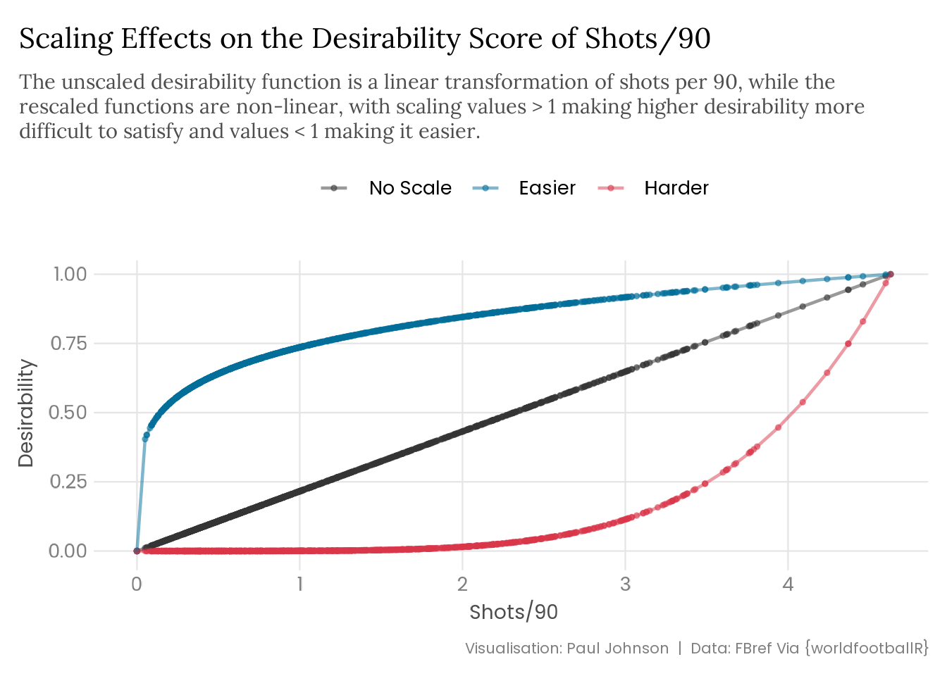
Scaling Desirability Functions
Each individual desirability function can be easily adjusted using the scaling feature, \(s\), which can be increased in order to make maximal desirability harder to reach, and decreased to make it easier. The default value is 1 because \(s\) is an exponent and a 1 effectively cancels this out. We’re having fun.
In the goal threat desirability function, goals and expected goals have \(s = 2\), while for shots and touches in the opponent’s penalty area \(s = 0.5\). This captures the fact that npG and npxG are very direct measures of goal threat (they are literally the actual goals and the probability of scoring actual goals!), while shots and touches are a lot less direct. I suspect we’d be better served giving shots greater weight in the function than touches, but in the interest of trying my hardest not to get bogged down in the domain context and focus on the method, let’s just give them the same weight.
Given that \(s\) is the exponent, the scaling feature transforms the desirability function in a non-linear manner. The plot below illustrates how scaling affects desirability.
Plot Code (Click to Expand)
big_five_stats |>mutate(# maximise shots90 without rescalingno_scale =d_max(sh90, use_data =TRUE),# maximise shots90 with lower scaleeasier =d_max(sh90, use_data =TRUE, scale =0.2),# maximise shots90 with higher scaleharder =d_max(sh90, use_data =TRUE, scale =5) ) |> tidyr::pivot_longer(cols =c(no_scale, easier, harder), names_to ="scaling", values_to ="value" ) |>mutate(scaling =factor(scaling, levels =c("no_scale", "easier", "harder"))) |>ggplot(aes(x = sh90, y = value, colour = scaling)) +geom_point(size =1, alpha = .5) +geom_line(linewidth =0.8, alpha = .5) +scale_colour_manual(values =c("grey20", "#026E99", "#D93649"),labels = snakecase::to_title_case ) +labs(title ="Scaling Effects on the Desirability Score of Shots/90",subtitle = stringr::str_wrap( glue::glue("The unscaled desirability function is a linear transformation of ","shots per 90, while the rescaled functions are non-linear, with ","scaling values > 1 making higher desirability more difficult to ","satisfy and values < 1 making it easier." ),width =95 ),x ="Shots/90", y ="Desirability",caption ="Visualisation: Paul Johnson | Data: FBref Via {worldfootballR}" )
When scaling desirability functions I think it is important to recognise the effects that imposing a non-linear transformation has. Because I’ve used the use_data = TRUE argument in d_max(), the maximum and minimum value in each desirability function is set by the data, meaning that regardless of the scaling applied the maximum value will still be 1 and the minimum value will be 0. However, as the scale increases, this will make it much harder for values to reach higher desirability scores, meaning that lower values of the corresponding variable will be given lower scores, but the non-linearity imposed increases the rate of desirability increases at higher values of the corresponding variable.
It is important to realise that making maximal desirability harder in this non-linear fashion does not downweight the highest values of that variable. Instead, it actually increases the magnitude of those highest values, because so few other observations are similarly high! Therefore, if you want to downweight the value of a particular variable in the overall desirability score, it needs to be easier to reach maximal desirability, because all values of that variable will have a higher score and that will give the highest values less leverage.
I think it is a little difficult to process the exponential effects of \(s\) in this context. We are primarily interested in the highest values of each desirability function, given that the focus is on building a rating system, and increasing \(s\) achieves our goals at the top-end of the ratings, but it obviously feels a little wonky to exponentially increase the value of a particular desirability function in order to downweight it in the overall desirability score! I think it is sensible to visualise the effects that your intended scaling will have, so as to help you think through the choices you’re making.
Chance Creation
If doing goals is the most important part of an offense in football, then helping others do goals must be the next best thing. Which brings us to chance creation. The process for creating a rating system for chance creation is more or less the same as with goal scoring. I’ve selected three variables that will go into the chance creation ratings - assists, expected assists (xA), and shot-creating actions (SCA).
In this case, the SCA desirability function has been scaled to reduce SCA’s effect on the overall score but assists and expected assists are unscaled. While I think that shot-creating actions are not quite as valuable as assists, I don’t want to exponentially increase the value of assists and expected assists at the top end of the desirability score. Goalscoring is the most important part of football, so I think small increases in the per 90 rate of goalscoring should be rewarded greatly, but creating chances, while still very important, is still reliant on the player receiving the ball putting it away, and I think the decisions made here reflect that.
Just as with the goal threat component, the choices I’ve made here are more of an art than a science, and I think I could easily be convinced that the way I’ve structured the desirability functions for chance creation are incorrect. Unfortunately for you, I’m not actually having that debate, so I went ahead and made my own choice. It’s probably wrong. Table 2 shows the results of my poor choices, in life and in this blog post.
Again, the names at the top of the Table 2 ratings give me confidence, especially the three names at the very top - Kevin De Bruyne, Neymar, and Lionel Messi. I don’t think there are any huge surprises in these ratings, perhaps with the exception of Rémy Cabella, who has some solid to very good creation numbers but wouldn’t necessarily be a name you’d immediately think of when thinking about the ten best creative players in the world. This is once again a reminder that Ligue 1 is very silly but is wonderfully chaotic.
Ball Progression
The final component, and possibly the most interesting of the three, is ball progression. The three variables included in the ball progression desirability function are progressive carries, passes, and receptions. Just as is the case with the previous two components, I’m sure you could include other variables as measures of ball progression, but I’m still too lazy to do that and I think a lot of those other variables would risk double-counting where those actions are picked up by one of the progression metrics.
I am particularly unsure about how to weight the value of progressive actions, especially progressive passing and receptions, which are connected actions. I could see an argument for giving less weight to progressive receptions, and treating carries and passes equally, but I could also see a case that progressive passes and receptions should be treated equally because both the passer and receiver have to do their job to make the progressive action successful. Given my uncertainty about this particular category, I’ve decided it is best to weight all three variables equally.
Forwards dominated the first two components but Table 3 is more diverse. This is to be expected, given that ball progression is often about moving the ball up the pitch to the forwards! Table 4 aggregates the ball progression desirability scores by position.
Table 4: Ball Progression Desirability by Position
Position
Desirability Scores
Progressive Carrying
Progressive Passing
Progressive Receptions
Overall
FW
0.31
0.16
0.39
0.26
MF
0.22
0.35
0.17
0.23
DF
0.16
0.24
0.12
0.18
Source: FBref Via {worldfootballR}
The results are not shocking, but the marginal differences in progression by position are interesting. As expected, forwards are dominant in the receptions category, but the responsibilities for progressive carries are more evenly split, and forwards are third behind midfielders and defenders in progressive passing.
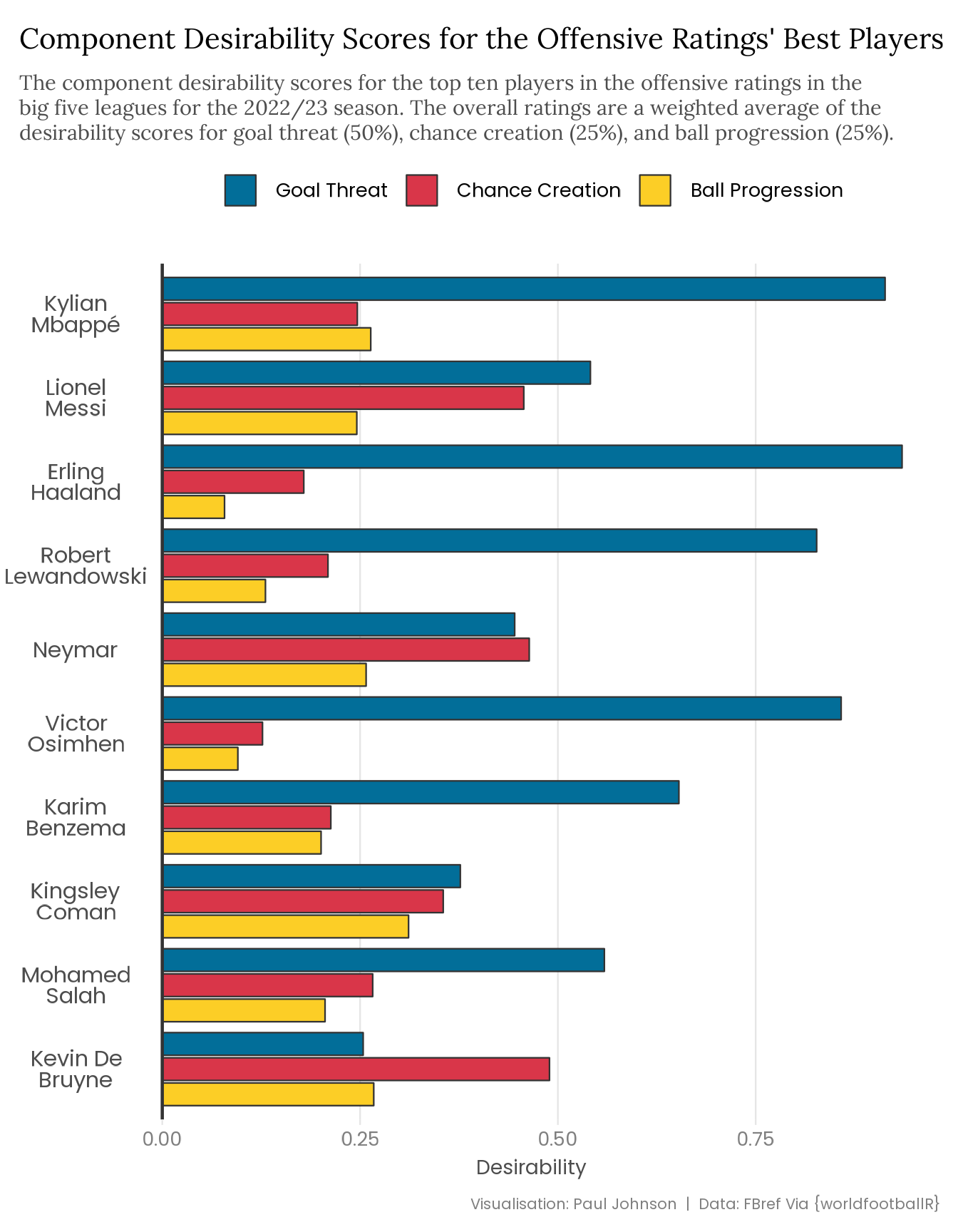
Overall Offensive Ratings
Having created desirability scores for each offensive component, we could combine all three into an overall offensive rating using d_overall(). I think this would be a reasonable choice when the assumption is that each category is equally important in the overall score, but as discussed already, I don’t think that’s the case here. I think goal threat matters most, and chance creation and ball progression are, while important enough to be the two other categories in the overall ratings, a little less important than goals.
Whether or not goals are more important than chance creation and ball progression is probably open to plenty of debate, but assuming that they are (because this is my blog and I said so), we have to weight the three categories to reflect this. Rather than overcomplicating things and trying to do this as part of the process within the desirability functions, I have downweighted chance creation and ball progression by multiplying them by 0.5.
Finally, I have opted for the arithmetic mean instead of the geometric mean, because I think the purpose of the geometric mean is of less value here.
The old rule was that any metric not broken by Lionel Messi being so far ahead of everyone else is wrong, but Messi isn’t quite the freak of nature he once was. Nonetheless, Messi’s name being near the top of the ratings is a good sign, as is Mbappé and Haaland flanking him at the top. At a glance, there are few surprises in Table 5.
Kingsley Coman making it into the top ten feels generous, but perhaps the biggest issue is the three Ligue 1 players in the top five. While those three players are exceptional, they seem to be rated a little too high. I think this points to the inevitable league effects compromising the ratings. The big five leagues have been treated equally and we know that isn’t really the case (Ligue 1 is probably the weakest of the five). A more precise approach would involve weighting by league strength, but that’s complicated and I don’t want to do it.
Nonetheless, I think the ratings look pretty reasonable, and when we split the top ten overall desirability scores into their component parts, visualised below, we can see how the three offensive components are balanced.
Plot Code (Click to Expand)
offensive_rating |>head(10) |> tidyr::pivot_longer(cols =5:7, names_to ="component", values_to ="value" ) |>mutate(component =factor( component, levels =c("Goal Threat", "Chance Creation", "Ball Progression") ) ) |>ggplot(aes(x =reorder(Player, Overall), y = value, fill = component)) +geom_col(position =position_dodge2(reverse =TRUE), colour ="grey20", linewidth =0.4) +geom_hline(yintercept =0, colour ="grey20", linewidth =0.8) +coord_flip() +scale_x_discrete(labels = scales::label_wrap(12)) +scale_fill_manual(values =c("#026E99", "#D93649", "#FCCE26")) +labs(title ="Component Desirability Scores for the Offensive Ratings' Best Players",subtitle = stringr::str_wrap( glue::glue("The component desirability scores for the top ten players in the ","offensive ratings in the big five leagues for the 2022/23 season. ","The overall ratings are a weighted average of the desirability scores ","for goal threat (50%), chance creation (25%), and ball progression (25%)." ),width =95 ),x =NULL, y ="Desirability",caption ="Visualisation: Paul Johnson | Data: FBref Via {worldfootballR}" ) +theme(panel.grid.major.y =element_blank(),axis.ticks.y =element_blank(),axis.text.y =element_text(colour ="grey30", size =rel(1.15), hjust =0.5, margin =margin(r =-15, l =-8), lineheight = .4 ) )
Limitations
I think the appeal of desirability functions is their simplicity, but this is also a constraint. As the complexity of the multivariate optimisation problem increases, the solutions will need to scale similarly. While desirability functions are a quick and easy optimisation method that can perform well in many contexts, I don’t think they’re suitable when dealing with the most complex, multidimensional problems. Developing a precise, reliable rating system for offensive players would probably involve doing something more complicated than desirability functions!
Scaling can improve the performance of desirability functions when dealing with complex optimisation problems, but deciding when and how to use them is difficult. It is more of an art than a science. Consequentially, scaling features risk encouraging searching for results that feel good. If you have theory-driven expectations of the weighted combination of a set of variables, you stand a better chance of avoiding results that confirm your biases but it is difficult to validate desirability functions outside of eyeballing the results and deciding whether they seem right.
Conclusion
I am generally pretty sceptical of player rating systems in football. Capturing a multidimensional context like this is difficult using a single measure of player performance. And yet here I am, developing a player rating system that attempts to do exactly that! In my defense, I have at least limited these ratings to offense, which makes it slightly better3, and it’s a lot easier to rate players over an entire season than a single match. But I’d take these results with a big pinch of salt. I would include several caveats if I released these ratings into the wild, for the non-nerds (there is no chance anyone but nerds is reading this). These ratings are going to be pretty noisy! That said, I don’t think the results are complete garbage, which meets the high standard I set for my work.
Hopefully, these ratings illustrate how desirability functions work and demonstrate that they could be appropriate in many situations. You don’t see desirability functions used very often, but they are quick and easy, and they can be pretty effective.
Kuhn, Max, and Kjell Johnson. 2019. Feature Engineering and Selection: A Practical Approach for Predictive Models. Taylor & Francis. https://bookdown.org/max/FES/.
Footnotes
With each variable \(X_i\) being simultaneously optimised, where \(i\) represents each individual variable, each must be individually optimised using a desirability function that approaches 1 when \(X_i\) is optimal and approaches 0 when \(X_i\) is unacceptable. The optimisation function for minimising \(X_i\)(Kuhn 2016) is given by:
where \(A_i\) and \(B_i\) specify the minimum and maximum value that each variable \(X_i\) can reach, and \(s_i\) is a scaling feature that makes it easier (\(s > 1\)) or harder (\(s < 1\)) for each variable \(X_i\) to achieve maximal desirability.
Similarly, the optimisation function for maximising variable \(X_i\)(Kuhn 2016) is:
where \(A_i\), \(B_i\), and \(s_i\) are again the minimum and maximum values and the scaling feature.↩︎
The arithmetic mean is the typical mean average value that people are used to seeing, which sums all values and divides the sum by the sample size, \(n\), while the geometric mean multiplies all values, before taking the \(n\)th root (the \(n\) being the number of values multiplied) of that product. Both arithmetic and geometric mean are measures of central tendency, but geometric mean is more robust when dealing with non-independent values, less responsive to outliers, and more capable of handling skewed data.↩︎
Defensive event data does not reflect performance and is more of a measure of team and player style.↩︎