In the opening post in the Missing Data Matters series1, I looked at the mechanisms that cause missing data - missing completely at random (MCAR), missing at random (MAR), and missing not at random (MNAR) - and demonstrated some of the options available for diagnosing missing data mechanisms. This post will cover the next step in the missing data workflow - what the hell are you supposed to do now, having realised that your data is complete trash?
I will use the same employee attrition dataset taken from the modeldata package and created by the IBM Watson Analytics Lab and will continue to add missingness to this data with reckless abandon. I will talk through the range of options available to you when faced with missing data, including both deletion and imputation methods, and I will also discuss how the missing data mechanism you are dealing with impacts the appropriateness of the available solutions. Finally, I will demonstrate how some of these methods work and compare their performance using a series of logistic regressions.
Have You Considered Not Having Missing Data?
The maximally optimal approach to missing data is to not have any, so if you have missing data, the best thing you can do is stop having it. The only way to do that is to go and find it! This may seem glib, but it’s important to highlight this point before looking at the other options. All of the strategies that are detailed below have drawbacks. If you can find your missing values, this is a much better choice than trying to model some solution. This may involve further data collection, identifying bugs/issues in your data processing pipeline, or theory-driven inference2.
However, when this is not possible, there are two broad approaches to dealing with missing values. The first approach is to delete missing values, and the second is to replace them. The right approach is highly dependent on the nature of the missing data. Generally speaking, data that is MCAR is the most flexible, and simple methods like deletion can work without problems, but more complex methods like imputation are necessary when data is MAR. Finally, when dealing with MNAR data, it is required to model the missingness mechanism explicitly (Gelman and Hill 2006).
A Quick Note on MNAR Data
Although we may touch on MNAR data in passing in this second post, the focus will be on MCAR and MAR data. The process for modelling MNAR data is complicated, and I am a massive coward. Cramming the suite of potential MNAR solutions into an already complex post would not do them justice.
However, as a quick summary, there are two main approaches to modelling MNAR data - selection modelling and pattern mixture modelling. Selection models treat missingness as the outcome in a regression, similar to a more precise version of the logistic regression fit in the previous post, while pattern mixture models treat the missingness as an explanatory variable.
For more information about MNAR modelling processes, I’d recommend Enders (2022)’s Applied Missing Data Analysis.
And Another on Likelihood Methods for Good Measure
One group of methods I haven’t discussed here is likelihood methods, such as full information maximum likelihood (FIML). In simple terms, likelihood methods borrow information from complete cases to improve the estimation of parameters with missing data (Peters and Enders 2002). Maximum likelihood uses the available information to estimate a log-likelihood function most likely to have produced the observed data (Enders 2022). In particular, FIML considers only complete cases when calculating the log-likelihood function and maximises it using an expectation-maximisation algorithm (Xu, Chen, and Li 2022).
However, implementing methods like FIML in R is a little tricky3, so these methods are out of scope for my rubbish little blog post. If you want to learn more about the implementation of FIML in R, I’d recommend the “Full Information Maximum Likelihood” section of William Murrah’s Statistical Thinking site and there the lavaan package documentation can also help figure out how to compute FIML to deal with missing data. If I am feeling like a total mad lad later on, I may write another post about implementing FIML.
Deletion Methods
The most straightforward and most common approach to handling missing data is to delete it. There are two different approaches to deleting missing values: listwise and pairwise deletion4.
Listwise deletion, sometimes called complete case analysis, is the most common. It removes any rows containing missing values for relevant variables. This means that the analysis is carried out on all complete cases. This is the default approach that almost every statistical tool in any language uses. It is the mechanism by which the plots in Part I of the series are visualising the different types of missing data5. When you choose not to resolve the missing data in your dataset, you are passing the buck and letting whatever statistical tool you are using do it for you, and they are usually carrying out listwise deletion.
Pairwise deletion, or available case analysis, is less common. It involves removing any missing values but not the entire row. Instead, the available observations for each variable are used to calculate their means and covariances, which can be used to build statistical models (Van Buuren 2018). This process is a little more involved and cannot be applied to as many use cases, so you should see pairwise deletion far less often in the wild.
Deletion-based methods can be robust under the right conditions. When data is MCAR and volumes of missing data are not vast, deletion methods may be suitable. However, things can start to unravel when data is MAR, and deletion methods will likely cause many problems when data is MNAR. Deleting values when data is MNAR (and to a slightly lesser extent MAR) creates selection bias. The sample that remains after deletion is a function of the missing data mechanism, which cannot be accounted for in a model if the data has been deleted. Nonetheless, deletion methods prevail because they are the default approach.
Imputation Methods
If we are not deleting missing values, we have to replace them. Imputation involves using a statistical procedure to replace missing values with values estimated from the rest of the data.
Imputation methods can be divided into single imputation and multiple imputation. Single imputation replaces missing values with a single value, while multiple imputation creates \(m\) datasets, each replacing missing values with plausible estimated values and pooling estimates from analyses carried out on each dataset.
Imputation is appropriate under the starting assumption that the data is MAR. It is also suitable when dealing with MCAR data, but deletion methods are usually most appropriate unless dealing with large volumes of missingness.
In addition to mice’s exploratory capabilities, it is also the go-to option for carrying out imputation in R6. While I will briefly overview these methods, there is much more to imputation than could be covered here. To learn just about all there is to know about imputation, Van Buuren (2018)’s Flexible Imputation of Missing Data will have you covered.
Single Imputation
There are a few different forms of single imputation, the most common being simple imputation methods that replace all missing values with the variable’s average value (usually the mean, but median and mode can be used too) or replace missing values using randomly drawn values from the same variable, otherwise known as simple hot-deck imputation (Xu, Chen, and Li 2022). Simple imputation methods are almost always harmful, especially methods like mean imputation. They distort the variable’s distribution, underestimating its variance (Van Buuren 2018), disrupting the relationship between the variable with imputed values and all other variables (Nguyen 2020), and biasing model estimates (Van Buuren 2018). It is important to know that these simple imputation methods exist, but the circumstances where using them is valid are very few!
Another approach is to estimate a regression model that predicts missing values. Regression imputation could take the form of any regression model, depending on the data type and complexity, with linear and logistic regression being the most common. However, Van Buuren (2018) argues that regression imputation is the “most dangerous” method because it gives false confidence in outputs.
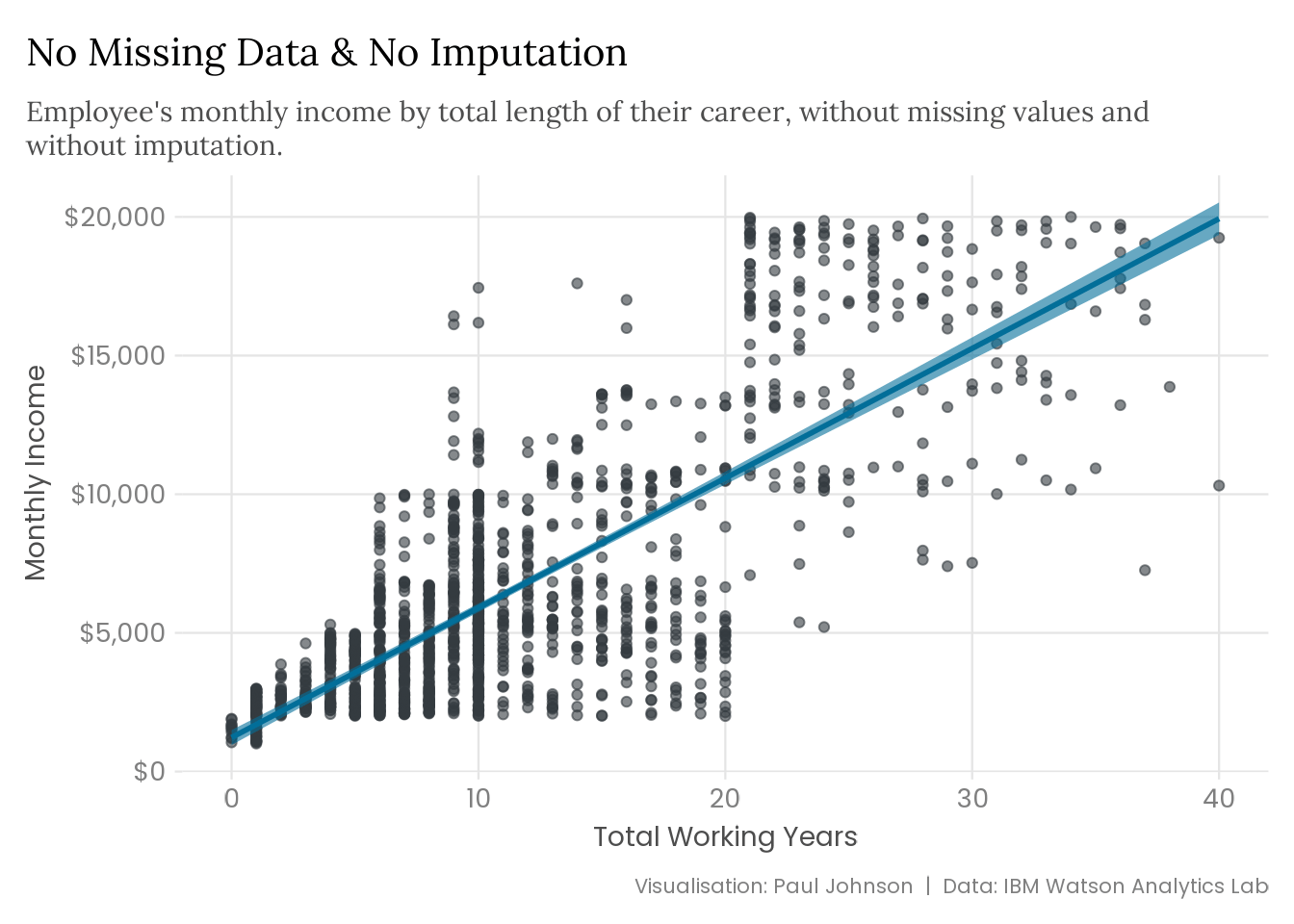
We can look at the effects of imputation by visualising imputation methods. I have transformed the total working years value for 75% of employees with high or very high relationship satisfaction to NA. Obviously, this is a very high proportion of missing values. If 75% of your data is missing, you should be deeply alarmed, stop whatever you are doing, and bin that dataset. However, in this case, it is meant to illustrate how imputation methods work, and having a disproportionately large number of missing values makes it easier to see the effects visually.
plot_regression <-function(data) {if ("missingness"%in%names(data)) { data |>ggplot(aes(x = total_working_years, y = monthly_income)) +geom_point(aes(colour = missingness), size =1.5, alpha = .6) +geom_smooth(method = lm, colour ="#026E99", fill ="#026E99", alpha = .6) +scale_colour_manual(values =c("#D93649", "#343A40")) +scale_y_continuous(labels = scales::label_currency()) +guides(colour =guide_legend(override.aes =list(size =3))) +labs(x ="Total Working Years", y ="Monthly Income",caption ="Visualisation: Paul Johnson | Data: IBM Watson Analytics Lab" ) } else { data |>ggplot(aes(x = total_working_years, y = monthly_income)) +geom_point(colour ="#343A40", size =1.5, alpha = .6) +geom_smooth(method = lm, colour ="#026E99",fill ="#026E99", alpha = .6 ) +scale_y_continuous(labels = scales::label_currency()) +labs(x ="Total Working Years", y ="Monthly Income",caption ="Visualisation: Paul Johnson | Data: IBM Watson Analytics Lab" ) } }attrition |>plot_regression() +labs(title ="No Missing Data & No Imputation",subtitle = stringr::str_wrap( glue::glue("Employee's monthly income by total length of their career, without ","missing values and without imputation." ),width =90 ) )
Plot Code (Click to Expand)
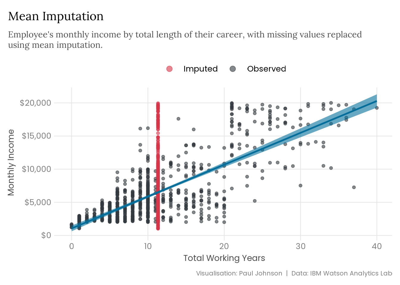
missing_years |> mice::mice(method ="mean", m =1,maxit =1, print =FALSE ) |> mice::complete() |>plot_regression() +labs(title ="Mean Imputation",subtitle = stringr::str_wrap( glue::glue("Employee's monthly income by total length of their career, with ","missing values replaced using mean imputation." ),width =90 ) )
Plot Code (Click to Expand)
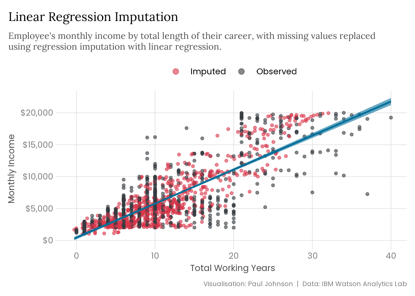
missing_years |> mice::mice(method ="norm.predict", m =1,maxit =1, print =FALSE ) |> mice::complete() |>plot_regression() +labs(title ="Linear Regression Imputation",subtitle = stringr::str_wrap( glue::glue("Employee's monthly income by total length of their career, with ","missing values replaced using regression imputation with linear ","regression." ),width =90 ) )
Imputing missing values using simple mean imputation is quick and easy, but the results clearly leave much to be desired. However, estimates can sometimes be useful even if they are imprecise. That’s not the case here either because mean imputation narrows the distribution of total working years. The confidence intervals around the regression line are narrower around the mean but significantly wider at the higher end of total working years.
The regression imputation is okay at first inspection, but it imputes values of total working years to six decimal points while the actual values are all integers. The imputation also thinks that some people have worked negative years! These issues can be fixed by giving mice the necessary details to impute more realistic values. However, the razor-thin error bars, particularly at the lower values of total working years, cannot be fixed using single imputation.
This points to the inherent flaw with single imputation that none of these methods can escape. In Rubin (1987)’s words:
Imputing one value for a missing datum cannot be correct in general, because we don’t know what value to impute with certainty (if we did, it wouldn’t be missing).
We cannot account for the uncertainty in imputing missing values using single imputation because we are plugging in a single value in place of the missing value and treating it with the same confidence as the observed values. There are ways to add more uncertainty to single imputation methods, such as stochastic regression imputation, but ultimately, these are papering over the cracks. Single imputation always offers a false sense of certainty because it imputes a single value in place of each missing value.
Multiple Imputation
Multiple imputation attempts to address the fundamental flaw in single imputation methods, acknowledging the uncertainty in imputed values and baking that uncertainty into the process. Multiple imputation involves generating multiple datasets, performing analysis on each, and pooling the results. The multiple imputation process yields parameter estimates that “average over a number of plausible replacement values” (Enders 2022, 189) instead of the one that single imputation does. Multiple imputation can be appropriate for missing data that is not MAR, as long as the response mechanism has been explicitly modelled or other identifying assumptions have been made (Murray 2018).
Enders (2022) splits the multiple imputation process into three phases - imputation, analysis, and pooling.
Imputation Phase - generates multiple, \(m\), complete datasets, estimating the missing values plus a random component to capture the uncertainty in the estimate,
Analysis Phase - computes parameter estimates using typical statistical methods, but computed \(m\) times and applied to the \(m\) completed datasets,
Pooling Phase - combines these estimates7 and calculates the pooled estimates and their standard errors.
While there are multiple ways to approach each phase, the three phases are typical across multiple imputation.
Here, we will use multiple imputation by chained equations (MICE). MICE imputes one variable at a time, using a separate model for each incomplete variable, a process called Fully Conditional Specification. Plausible values are generated using the rest of the data columns (using various methods depending on the variable) in an iterative process that uses Gibbs sampling (Van Buuren and Groothuis-Oudshoorn 2011).
Effective multiple imputation requires as much information as possible, including variables associated with the missingness itself and with the observed values of that variable (which are, therefore, likely to be associated with the missing values). Thus, Murray (2018) argues that imputation models should include as many variables as possible.
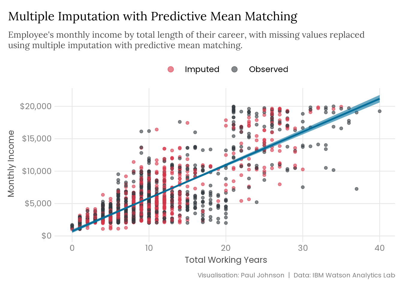
The plot below shows the results of the imputation phase of the multiple imputation process, with the pooling carried out manually, but it is important to note that the results are not a perfect implementation of multiple imputation. Instead, each of the five completed datasets has been stacked together, and the mean value of each row8 across those five datasets has been calculated. The results plotted below do not perfectly demonstrate what multiple imputation looks like, but they are at least an approximation.
Plot Code (Click to Expand)
missing_years |> mice::mice(method ="pmm", print =FALSE, seed =123) |> mice::complete(action ="long") |>summarise(across(c(total_working_years, monthly_income), ~round(mean(.x), 0)), .by =c(.id, missingness) ) |>plot_regression() +labs(title ="Multiple Imputation with Predictive Mean Matching",subtitle = stringr::str_wrap( glue::glue("Employee's monthly income by total length of their career, with missing ","values replaced using multiple imputation with predictive mean matching." ),width =90 ) )
The confidence intervals don’t capture the baked-in uncertainty, a significant advantage of multiple imputation. The plot only shows the final mean values calculated from the five imputed datasets. However, the multiple imputation process results follow a similar distribution to the original data, which should reduce the risk of imputations producing biased parameter estimates. Further, the imputed values appear to be structured similarly to the observed data, making the multiple imputation plot look very similar to the original data plot. This is generally a good sign because the closer you are to replicating the data-generating process, the better your chance of making accurate inferences. The structural similarities are primarily due to the method used to carry out the multiple imputation, predictive mean matching.
Predictive Mean Matching
The method used for modelling plausible values is predictive mean matching (PMM). PMM estimates missing values by identifying candidates from the observed data with predicted values close to the missing observation’s predicted value, from which a candidate is randomly selected and the observed value is plugged in the missing observation’s place (Van Buuren 2018). Predictions are typically generated using a linear regression model. PMM effectively identifies \(n\) observations from the observed data closest to the predicted value of the missing data and picks one at random.
There are several advantages to using PMM. Implementation is simple; it relies on imputations that are observed elsewhere in the data (which ensures it is realistic and won’t produce nonsensical imputations), and because the imputation process is implicit, it doesn’t require explicit modelling of the missingness distribution and, therefore reduces the risk of misspecification (Van Buuren 2018). A more detailed discussion of PMM can be found in the “Predictive Mean Matching” section of Van Buuren (2018)’s Flexible Imputation of Missing Data.
While I’ve used PMM here, mice offers functionality for various methods for multiple imputation. In this case, the missing values are all numeric, for which mice uses PMM as the default imputation method. However, for binary factor variables, logistic regression is used by default, and where a factor variable has more than two levels, proportional odds regression is used when it is ordered, and polytomous logistic regression is used when it is unordered.
Comparing Model Estimates
Finally, we can test these missing data methods by fitting regression models using them. We can compare the model estimates with each other and against a regression fit on the original data.
I have fit a series of logistic regressions that measure the association between the outcome, job attrition, and the explanatory variables monthly income, total working years, and number of companies worked. All explanatory variables have been transformed to include some missingness. The missing data mechanism in each case is MAR. Monthly income values have been converted to NA for 75% of research scientists or sales executives educated to a Bachelor’s degree or higher. For total working years, 75% of employees between 50 and 60 have been converted to NA. Finally, the number of companies an employee has worked at has been converted to NA for 25% of employees with low job satisfaction.
I have used the defaults for most imputation processes, but I have increased the number of iterations that the Gibbs sampler uses from 5 to 10 and have increased the number of complete datasets generated by the multiple imputation process from 5 to 30. While earlier literature on the subject argues that a small number of imputations (typically 3-5 total) is better, Van Buuren (2018) lays out the case for increasing the number of imputations, where computational cost is not a problem, in the “How Many Imputations?” section of Flexible Imputation of Missing Data.
Regression Code (Click to Expand)
get_pooled_estimates <-function(data, method, m, maxit) {if(m >1) { data |> mice::mice(method = method, m = m, maxit = maxit, print =FALSE, seed =123 ) |>with(glm(attrition ~ monthly_income + total_working_years + num_companies_worked, family ="binomial") ) |> mice::pool() } else { data |> mice::mice(method = method, m = m, maxit = maxit, print =FALSE) |> mice::complete() |>glm(attrition ~ monthly_income + total_working_years + num_companies_worked, family ="binomial", data = _) } }original_glm <- attrition |>mutate(monthly_income = arm::rescale(monthly_income)) |>glm(attrition ~ monthly_income + total_working_years + num_companies_worked, family ="binomial", data = _)listwise_deletion <- missing_income |>glm(attrition ~ monthly_income + total_working_years + num_companies_worked, family ="binomial", data = _)mean_imputation <- missing_income |>get_pooled_estimates(method ="mean", m =1, maxit =1)regression_imputation <- missing_income |>get_pooled_estimates(method ="norm.predict", m =1, maxit =1)multiple_imputation <- missing_income |>get_pooled_estimates(method ="pmm", m =50, maxit =10)
More can be done to tailor and tighten up mice’s imputations, but the intention here is only to demonstrate how different missing data methods perform out of the box.
While the imputations visualised in Section 3.2 are only an approximation of the process, the outputs displayed in Table 1 below fully demonstrate the multiple imputation method.
Table 1: Logistic Regressions Using Different Missing Data Strategies
Outcome: Job Attrition
Original Data
Listwise Deletion
Imputation
Mean
Regression
Multiple
(Intercept)
0.260
0.297
0.247
0.261
0.262
(0.052)
(0.082)
(0.047)
(0.056)
(0.058)
Monthly Income
0.574
0.387
0.334
0.520
0.543
(0.161)
(0.166)
(0.095)
(0.163)
(0.174)
Total Working Years
0.937
0.906
0.931
0.932
0.933
(0.017)
(0.023)
(0.017)
(0.017)
(0.018)
Num Companies Worked
1.107
1.097
1.114
1.117
1.111
(0.032)
(0.041)
(0.033)
(0.033)
(0.033)
Num.Obs.
1470
989
1470
1470
1470
Num.Imp.
50
Source: IBM Watson Analytics Lab
Table 1 highlights how impressive multiple imputation can be and why it is often ill-advised to use deletion or single imputation methods. While there are one or two coefficients where the deletion or single imputation methods are close to or even marginally outperform the multiple imputation process, the multiple imputation results are significantly better overall.
It’s not only that the coefficient estimates are generally closer to the estimates on the original data but also that the standard errors account for the greater uncertainty that should be factored in when imputing missing values. This is good. We do not want to be overconfident in conclusions drawn on data that includes imputed values, and multiple imputation guards against this.
Which Way, Western Man?
So, what kind of analyst are you going to be? Are you going to impute everything because unbiased estimates are overrated? Or will you delete all your missing data because less data is good, and there couldn’t be anything important in those observations anyway? The good news is that these are improvements compared to what you have probably been doing until now. Not dealing with missing values is a methodological choice in and of itself, often a bad one. Sometimes, listwise deletion is defensible, but you should be the one to make that call because you’re the one who’s on the hook for the consequences! As Newman (2014) argue - abstinence is not an option.
Of course, if you want to show everyone what a wise old sage you are, consider multiple imputation instead.
This blog post only scratches the surface of missing data methods. As tempting as it might be to summarise an entire research field, I’d also have to read about 2,000 Donald Rubin papers before I could even get started on what anyone else has to say on this topic. Various methods, such as likelihood methods and multilevel imputation, haven’t been covered here, and I haven’t discussed the evaluation of imputation results. All of this stuff is important! But this blog post is already longer than I originally planned, and if I’m not careful it’ll soon end up being so large that tech companies will start using it as a corpus to train their large language models. Hopefully, this brief introduction will inspire you to continue learning about missing data methods.
Acknowledgments
Many thanks to Camilo Alvarez (of the great Trivote Discord fame) for his kind but constructive feedback during the development of this series of blog posts. I greatly appreciate anyone who helps me be just a little less stupid.
The preview image was generated using StabilityAI’s DreamStudio, using the prompt “An eerie-looking image of a boy lost in a field, with a sign behind him saying ‘Missing Data - Please Return At Earliest Convenience’”.
Enders, Craig K. 2022. Applied Missing Data Analysis. Guilford Publications.
Gelman, Andrew, and Jennifer Hill. 2006. “Missing-Data Imputation.” In Data Analysis Using Regression and Multilevel/Hierarchical Models, 529–44. Cambridge University Press.
Peters, Cara Lee Okleshen, and Craig Enders. 2002. “A Primer for the Estimation of Structural Equation Models in the Presence of Missing Data: Maximum Likelihood Algorithms.”Journal of Targeting, Measurement and Analysis for Marketing 11: 81–95.
Rubin, Donald B. 1987. Multiple Imputation for Nonresponse in Surveys. Wiley.
Van Buuren, Stef, and Karin Groothuis-Oudshoorn. 2011. “MICE: Multivariate Imputation by Chained Equations in r.”Journal of Statistical Software 45 (3): 1–67. https://doi.org/10.18637/jss.v045.i03.
Xu, Tianchen, Kun Chen, and Gen Li. 2022. “The More Data, the Better? Demystifying Deletion-Based Methods in Linear Regression with Missing Data.”Statistics and Its Interface 15 (4): 515.
Footnotes
I keep calling it a series because I couldn’t think of another way to refer to it, but calling two posts a series feels grandiose. Am I forgetting a better word for this?↩︎
If you know the data well and can identify precisely why the data is missing, you may also be able to plug in the missing values. However, you should be pretty sure when doing this because otherwise, you have personally taken the time to add some error to your data. This is bad for all but the most graft-thirsty High Performance Podcast listening maniacs. If you would take the $500k over dinner with Jay-Z, you should make sure your theory is sound!↩︎
Or is at least sufficiently distinct from the implementation of the methods discussed below that it would be significant work to include likelihood methods in this post.↩︎
As I type this, it occurs to me that there are probably more than two methods for deleting missing values. Maybe someone out there advocates deleting the whole dataset and smashing your laptop with a hammer whenever you encounter NAs.↩︎
ggplot2 removes NAs by default, so the plots in the previous post are working by creating missing values and letting ggplot2 do the rest.↩︎
For anyone that prefers to use Python, statsmodels also has the functionality for multiple imputation by chained equations, while fancyimpute and sklearn.impute offer further imputation functionality.↩︎
Rubin (1987) devised formulas for pooling parameter estimates and standard errors, where the pooled parameter estimate is the arithmetic mean of the individual estimates, while pooled standard errors follow a similar logic but a slightly more complex process (Enders 2022). There are also methods for calculating statistical significance, but things are getting much more complicated now, and this is not the time or the place. I’d recommend reading “The Analysis and Pooling Phases of Multiple Imputation” in Enders (2022)’s Applied Missing Data Analysis if you want to get in the weeds.↩︎
The mean value has been rounded to the integer value so as to not mask what predictive mean matching is doing.↩︎